The numerical sensors are provided by the libUtil library. They allow to monitor any numerical values and write them in a separated file. Using the sensors requires two steps :

• initializing sensors. It consists in “placing” the numerical sensors to monitor the required values.

• triggering sensors acquisition with the _WriteSensorData standard plugin that collects sensor values and writes them in a file during the processing loop.

Prerequisites

You must follow the previous tutorial step before starting this tutorial. You need the simple tensile test built in the previous tutorial step.

Goal

It is proposed here to use sensors for monitoring the iteration number and the displacement of the “left” discrete element set.

Initializing sensor

To initialize sensors, a new plugin will be used. As it was previously shown, you can use the granoo3-project tool to build a new plugin from scratch.

:prompt: granoo3-project -p --cpp
Adding a new plugin...
PlugIn Name ? -> InitSensor
Do you want comments ? [(y)es or (n)o] -> n
-  Adding "PlugIn_InitSensor.cpp" file to the current dir
-  Adding "PlugIn_InitSensor.hpp" file to the current dir
-> Good bye ! 

#ifndef _PlugIn_InitSensor_hpp_
#define _PlugIn_InitSensor_hpp_

#include "GranOO3/Common.hpp"
#include "GranOO3/Core/PlugIn.hpp"

class PlugIn_InitSensor: public Core::PlugInInterface<PlugIn_InitSensor>
{
public: 
  DECLARE_CUSTOM_GRANOO_PLUGIN(InitSensor);

  PlugIn_InitSensor();
  ~PlugIn_InitSensor();

  void parse_xml();
  void init();
  void run();
};
#endif

#include "PlugIn_InitSensor.hpp"

REGISTER_GRANOO_PLUGIN(PlugIn_InitSensor);

PlugIn_InitSensor::PlugIn_InitSensor() 
  :Core::PlugInInterface<PlugIn_InitSensor>() {
}

PlugIn_InitSensor::~PlugIn_InitSensor() {
}

void
PlugIn_InitSensor::parse_xml() {
}


void
PlugIn_InitSensor::init() {
}


void
PlugIn_InitSensor::run() {
     // Get the time instance (the Time class is singleton)
  Physic::Time& time = Physic::Time::get();
  // Create a new sensor that catches the iteration number
  Core::Sensor::new_object(time, &Physic::Time::iteration, "Iteration");
 
  // Get the discrete element set named "left"
  Core::SetOf<DEM::DiscreteElement>& leftSet = Core::SetOf<DEM::DiscreteElement>::get("left");
  // Get the 0th element of this set
  DEM::DiscreteElement& el = leftSet(0);
  // Create a new sensor that catches its position vector 
  Core::Sensor::new_object(el, &DEM::DiscreteElement::get_position, "Position");
}

:prompt: granoo3-project -p --py
Adding a new plugin...
PlugIn Name ? -> InitSensor
Do you want comments ? [(y)es or (n)o] -> y
-  Adding "PlugIn_InitSensor.py" file to the current dir
 - Some lines were added to your 'Main.py' file
-> Good bye ! 

import granoo3.lib as granoo

class InitSensor(granoo.plugin):

    def __init__(self):
        granoo.plugin.__init__(self, "InitSensor")
        
    def run(self):
        # get the time instance (the Time class is singleton)
        time = granoo.time.get()
        # create a new sensor that monitors iteration number
        granoo.sensor.add(time.get_it, "Iteration")
 
        # get the discrete element set named "left"
        leftSet = granoo.discrete_element_set.get("left")
        # get the first element of this set
        el = leftSet.first()
        # Create a new sensor that catches its position vector 
        granoo.sensor.add(el.get_pos, "Position")  
        

In this example, only the run() run(self) method of the plugin is used. Two numerical sensors were created. The first one monitors the iteration number and the second one monitors the position of the discrete element placed at left. Numerical sensors are built with the static method that takes : an object, a pointer to a class method of this object and a string used to labeled the sensor. Be aware, never use temporary object here ! Because the object must be alive when the sensors is triggered with the WRITE-SENSOR-DATA plugin.

To avoid any further problems, do not use any special characters or white space in sensor labels.

Building and running

In order to execute the InitSensor plugin, you must add the following line in your tensile.inp file at the end of the PreProcessing section.

<InitSensor/>

In addition, you must add the following line at the end of the Processing section.

<WRITE-SENSOR-DATA/>

:prompt: cd build/ && cmake ../ && make && cd ../
:prompt: ./build/my-project.exe ./tensile.inp

:prompt: python ./Main.py ./tensile.inp

If you take a look at the Output directory, it must contain a Sensors.txt. This file must look like

Iteration	Position_X	Position_Y	Position_Z
0	1.0000000000e+00	0.0000000000e+00	0.0000000000e+00	
1	1.0000008665e+00	0.0000000000e+00	0.0000000000e+00	
2	1.0000034491e+00	0.0000000000e+00	0.0000000000e+00	
3	1.0000085639e+00	0.0000000000e+00	0.0000000000e+00	
4	1.0000169788e+00	0.0000000000e+00	0.0000000000e+00	
5	1.0000294004e+00	0.0000000000e+00	0.0000000000e+00	
...

Plotting your result

There is a lot of software solutions to plot this kind of file : spreadsheet softwares or scripting solutions such as gnuplot or matplotlib. Among these solutions, GranOO embeds a useful python script that allows easy plotting of the Sensors.txt files.

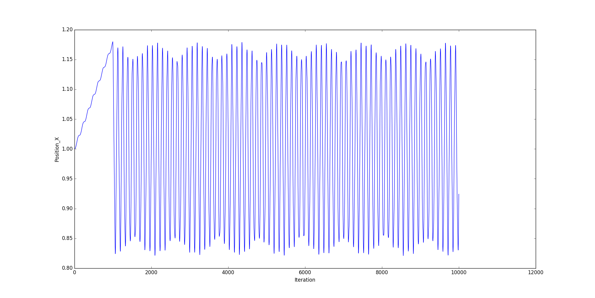
This script is named granoo3-plot. It uses the well known python matplotlib library. You can display a help message with the -h option as follows. The following command plots the position along X versus iteration number.

:prompt: granoo3-plot -f ./Tensile-test/Sensors.txt -x Iteration -y Position_X --run

It gives the following chart

Post-treating the “Sensors.txt” file

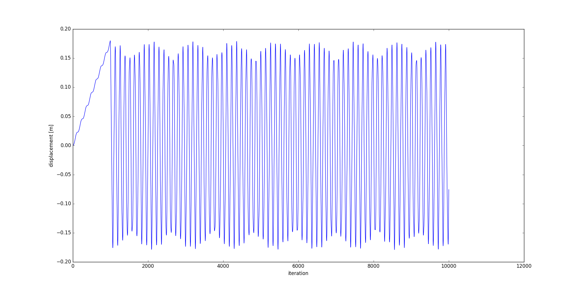
The previous section has plotted the position of the “right” discrete element along the X axis versus the iteration number. Now, we want to plot the displacement along the X axis. To do that, we need to post-treat the Sensors.txt file. To compute the displacement, the initial value of the position, given by the sensor, must be subtracted to each measured position values.

The granoo3-plot script can be used also as a python module. This module embeds useful functions that help users to post-treat and to plot a Sensors.txt file. The following python script named Plot.py shows how to :

• import the granoo3-plot script file as a module,
• parse the Sensors.txt file,
• store the read values as numpy arrays,
• do mathematic operations on these arrays and
• plot the result with matplotlib.

Now, you can create a new python file named plot.py that contains

# import granoo-plot
import granoo3.plot as gplot

# Import some useful modules
import matplotlib.pyplot as plt

# open and read the data file specified by the -f option
gplot.parseDataFile()

# now, we can use the column label as attribute name to access data.
# the data type are numpy arrays.
# the following example compute the displacement
iteration = gplot.data.Iteration
position  = gplot.data.Position_X
initial_position = position[0]
displacement     = position - initial_position

# plot the evolution of the displacement
fig = plt.figure()
plt.plot(iteration, displacement)
plt.xlabel('iteration')
plt.ylabel('displacement [m]')
plt.show()

If you run this script with the following command

:prompt: python ./py/plot.py -f ./Tensile-test/Sensors.txt

It gives the following chart